Optimization with PyGMO

The following paragraphs will give some information on how to optimize an astrodynamics problem written with tudatpy through the usage of PyGMO. The aim of this page is not to provide comprehensive documentation to the usage of PyGMO (such a guide already exists, see previous link), but rather to introduce the reader to the logic behind PyGMO and illustrate how to employ it jointly with tudatpy.

About PyGMO

The “basic” idea

PyGMO is a Python scientific library derived from PaGMO (Parallel Global Multiobjective Optimization), an open-source software developed at the European Space Agency by F. Biscani and D. Izzo [Biscani2020]. The flexible and complete framework of PaGMO (and of its equivalent PyGMO) can be applied to “single-objective, multiple-objective, continuous, integer, box-constrained, non linear constrained, stochastic, deterministic optimization problems”. Both programs are based on the concept of the island model, which in short is a computational strategy that allows to run the optimization process in parallel (hence its name) by using multithreading techniques.

Installing PyGMO

PyGMO is not part of the standard tudatpy distribution, but it can easily be added to any tudatpy environment. Here we will assume that you already have a standard tudatpy environment (called tudat-space) installed. If that is not the case, please follow the “Installing Tudat(Py)” instructions in Installation.

In order to make PyGMO available inside the tudat-space environment, the following steps need to be taken. First, activate the tudat-space environment:

$ conda activate tudat-space

Next, use conda to install the PyGMO package to this environment:

(tudat-space) $ conda install pygmo

Warning

Please ensure to install PyGMO in your given tudatpy environment. Do not add the PyGMO package to your base environment.

Note

If adding pygmo to an existing conda environment returns errors, create a new conda environment with pygmo added as a dependency.

name: tudat-space
channels:
  - conda-forge
  - tudat-team
dependencies:
  - tudatpy
  - matplotlib
  - scipy
  - pandas
  - jupyterlab
  - pygmo # <-- Add this line to your environment.yaml

Lastly, you should verify that the package is now available in your tudatpy environment. You can do so via your IDE or by using the following command in your terminal:

(tudat-space) $ conda list | grep pygmo

which should return the name, version, build and channel of the pygmo installation in the given environment.

First steps

There are a number of basic elements concurring to the solution of an optimization problem using PyGMO. These will be listed below and briefly explained; each of them correspond to an equivalent base class in PyGMO.

1. A problem. This represents the problem for which an optimal solution must be found. This is usually known, in PyGMO terminology, as User-Defined Problem (UDP); it is usually more interesting to code and solve a custom problem, but there are certain problems that are defined within PyGMO and can be readily used.

2. An algorithm. This is the procedure to solve the optimization problem. Similarly, this is known as User-Defined Algorithm (UDA); differently from the problem, it is often more convenient to take advantage of the many UDAs offered by PyGMO. Nonetheless, it is always possible to code a custom solver.

3. One (or more) individuals. Optimizers rely not on one, but many decision vectors that may interact (heuristic optimizers) or may not (analytical solvers) interact with each other. A set of individuals form a population. In PyGMO, it is more frequent to deal with an entire population, rather than with a single individual.

There are also two other fundamental blocks that conclude the structure of the island model. One is the island itself, which represents the main parallelization block to achieve simultaneous computation; the other one is the archipelago, consisting of a set of islands. These are useful to solve more advanced and computationally-demanding problems, therefore their usage will not be analyzed in detail here.

Optimizing a simple problem

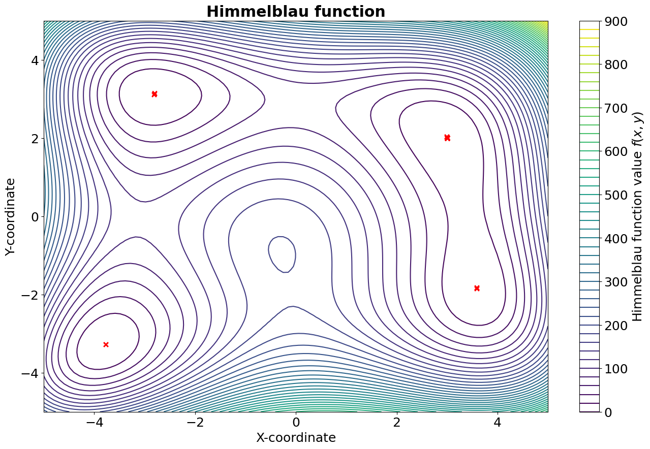
In this example, we will attempt to optimize a simple problem: the minimization of a known analytical function. We chose Himmelblau’s function as it is often employed to test the performance of optimization algorithms:

\[f(x,y) = (x^2 + y - 11)^2 + (x + y^2 - 7)\]

subject to the bounds:

\[\begin{split}\begin{align*} &-5 < x < 5 \\ &-5 < y < 5 \end{align*}\end{split}\]

There are four equal minima which can be found analytically. These are:

\[\begin{split}\begin{align*} f(3, 2) &= 0 \\ f(−2.805118,3.283186) &= 0 \\ f(−3.779310,−3.283186) &= 0 \\ f(3.584458,−1.848126) &= 0 \end{align*}\end{split}\]

Below, we will explain how to write the code for this specific UDP and solve it with PyGMO. The original code, which is broken down into parts for the sake of clarity, is available here.

1. Creation of the UDP class

First, we create a Python class to describe the problem. This class will be fed later to PyGMO, therefore it must be compatible. To be PyGMO-compatible, a UDP class must have two methods:

• fitness(np.array): it takes a vector of size \(n\) as input and returns a list with \(p\) values as output. \(n\) and \(p\) are respectively the dimension of the problem (in our case, \(n = 2\)) and the number of objectives (in our case, \(p = 1\) because it is a single-objective optimization).

• get_bounds(): it takes no input and returns a tuple of two \(n\)-dimensional lists, defining respectively the lower and upper boundaries of each variable. The dimension of the problem (i.e. the value of \(n\)) is automatically inferred by the return type of the this function.

import math

class HimmelblauOptimization:
    """
    This class defines a PyGMO-compatible User-Defined Optimization Problem.
    """

    def __init__(self,
                 x_min: float,
                 x_max: float,
                 y_min: float,
                 y_max: float):
        """
        Constructor for the HimmelblauOptimization class.
        """
        self.x_min = x_min
        self.x_max = x_max
        self.y_min = y_min
        self.y_max = y_max

    def get_bounds(self):
        """
        Defines the boundaries of the search space.
        """
        return ([self.x_min, self.y_min], [self.x_max, self.y_max])

    def fitness(self,
                x: list):
        """
        Computes the fitness value for the problem.
        """
        function_value = math.pow(x[0] * x[0] + x[1] - 11.0, 2.0) + math.pow(x[0] + x[1] * x[1] - 7.0, 2.0)
        return [function_value]

See also

For more information, see the PyGMO documentation about defining an UDP class.

2. Creation of a PyGMO problem

Once the UDP class is created, we must create a PyGMO problem object by passing an instance of our class to pygmo.problem. Note that an instance of the UDP class must be passed as input to pygmo.problem() and NOT the class itself. It is also possible to use a PyGMO UDP, i.e. a problem that is already defined in PyGMO, but it will not be shown in this tutorial. In this example, we will use only one generation. More information about the PyGMO problem class is available on the PyGMO website.

import pygmo

# Instantiation of the UDP problem
udp = HimmelblauOptimization(-5.0, 5.0, -5.0, 5.0)

# Creation of the pygmo problem object
prob = pygmo.problem(udp)

3. Selection of the algorithm

Now we must choose a specific optimization algorithm to be passed to pygmo.algorithm. For this example, we will use the Differential Evolution algorithm (DE). Many different algorithms are available through PyGMO, including heuristic methods and local optimizers. It is also possible to create a User-Defined Algorithm (UDA), but in this tutorial we will use an algorithm readily available in PyGMO. Since the algorithm internally uses a random number generator, a seed can be passed as an optional input argument to ensure reproducibility.

See also

For more information, see the PyGMO documentation about available algorithms and the PyGMO algorithm class.

Note

During the actual optimization process, fixing the seed is probably what you do not want to do.

# Define number of generations
number_of_generations = 1
# Create Differential Evolution object by passing the number of generations as input
de_algo = pygmo.de(gen=number_of_generations)
# Create pygmo algorithm object
algo = pygmo.algorithm(de_algo)

4. Initialization of a population

As a final preliminary step, a population of individuals must be initialized with pygmo.population. Each individual has an associated decision vector which can change (evolution), the resulting fitness vector, and an unique ID to allow their tracking. The population is initialized starting from a specific problem to ensure that all individuals are compatible with the UDP. The default population size is 0; in this example, we use 1000 individuals. Similarly to what was done for the algorithm, since the population initialization is random, a seed can be passed as an optional input argument to ensure reproducibility.

# Set population size
pop_size = 1000
# Set seed
current_seed = 171015
# Create population
pop = pygmo.population(prob, size=pop_size, seed=current_seed)

See also

For more information, see the page from the PyGMO documentation about the PyGMO population class.

5. Evolve the population

To actually solve the problem, it is necessary to evolve the population. This can be done by calling the evolve() method of the pygmo.algorithm object. We do so 100 times in a recursive manner. At each evolution stage, it is possible to retrieve the full population through the get_x() method and, analogously, the related fitness values with get_f(). If we are only interested in the best individual of each evolution stage, we can find its index through the pop.best_idx() method. On the contrary, the champion_x (and the related champion_f) attributes retrieves the decision variable vector and its fitness value. Note that the champion is the best individual across all evolutionary stages (not necessarily the best individual found at the last evolution).

# Set number of evolutions
number_of_evolutions = 100
# Initialize empty containers
individuals_list = []
fitness_list = []
# Evolve population multiple times
for i in range(number_of_evolutions):
    pop = algo.evolve(pop)
    individuals_list.append(pop.get_x()[pop.best_idx()])
    fitness_list.append(pop.get_f()[pop.best_idx()])

See also

For more information, see the PyGMO documentation about evolving a PyGMO population.

6. Visualization of the results

In the following figure, a contour plot of the Himmelblau’s function is reported, where the red X represent the best individuals of each generation. As it can be seen, the algorithm manages to locate all four identical minima.

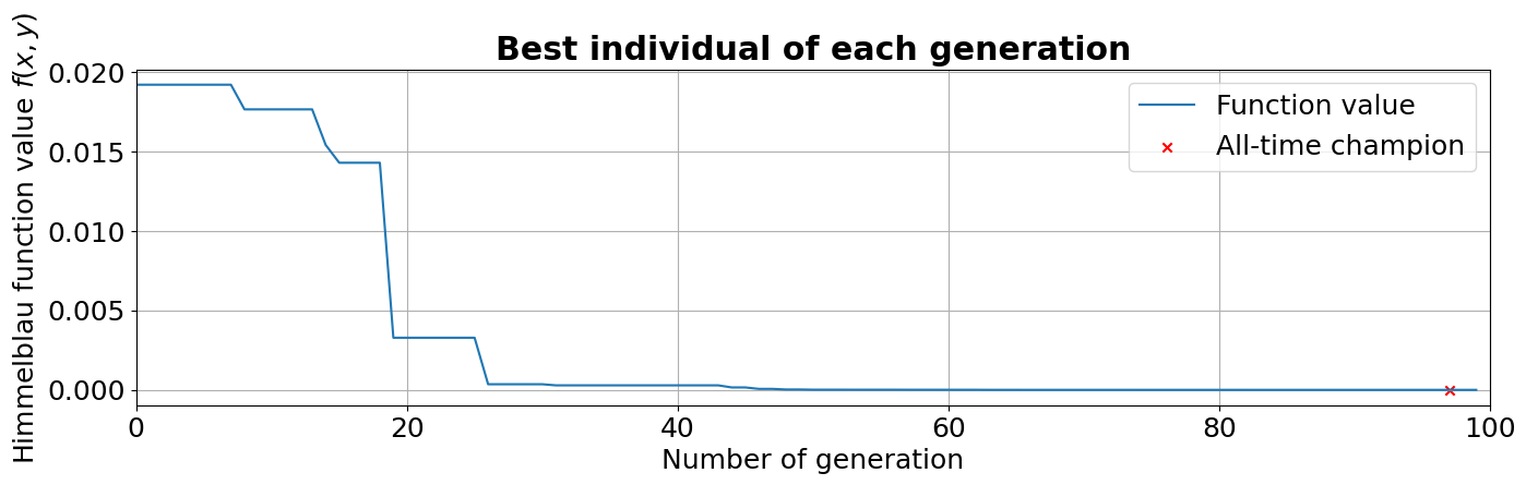
In the plot below, instead, we can see how the fitness of the best individual improves while the population is evolved. It can be seen, as anticipated before, that the champion is found a few generations before the last one.

The figure below illustrates indicatively the performance of the algorithm in the vicinity of one of the four minima.

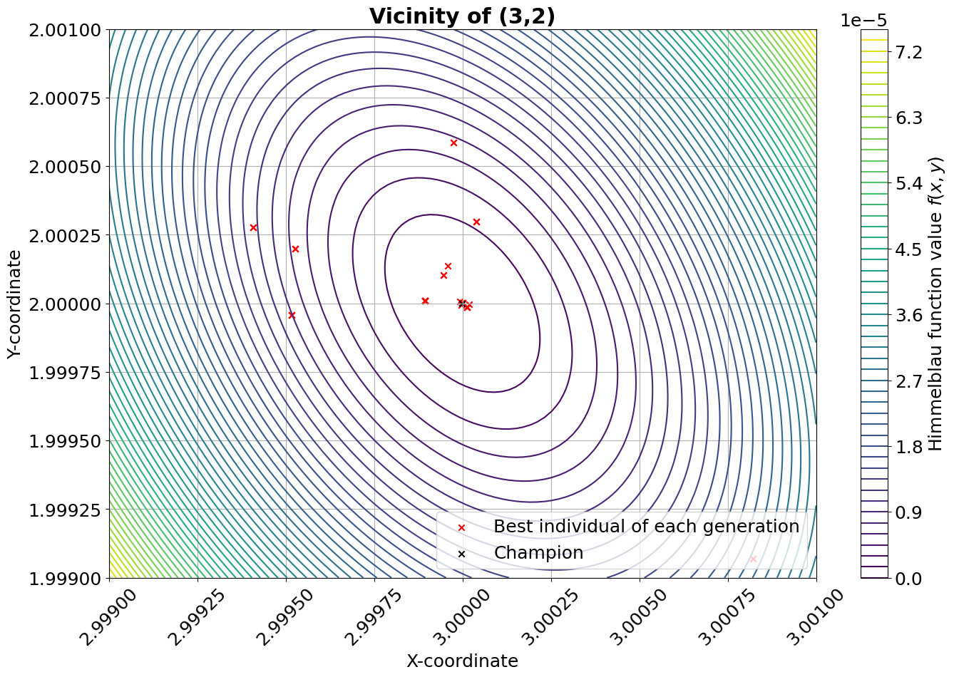
7. Performance of the algorithm

Since this is supposed to be an introductory example, a performance analysis of the algorithm is not presented here. However, it is interesting to provide a quick comparison between the optimization conducted with PyGMO’s DE algorithm two other simple analytical methods, namely a grid search and a Monte-Carlo search (both of them were run with 1000 points per variable). In the table below, referred to the minimum located at (3,2), the results are summarized in terms of accuracy and computational expenses. As it can be noticed, the DE algorithm reaches a fitness level several orders of magnitude below the other two methods, despite using only 10% of the computational resources.

Optimization method	Fitness value	Decision variable difference wrt (3,2)	Function evaluations
PyGMO’s DE (100 gens, 1000 individuals)	\(1.292 \cdot 10^{-11}\)	\((-6.365 \cdot 10^{-7}, +2.382 \cdot 10^{-7})\)	\(1.01 \cdot 10^{5}\)
Grid search (1000 points per variable)	\(4.215 \cdot 10^{-4}\)	\((-2.002 \cdot 10^{-3}, -3.003 \cdot 10^{-3})\)	\(1.00 \cdot 10^{6}\)
Monte-Carlo search (1000 points per variable)	\(7.095 \cdot 10^{-4}\)	\((+4.595 \cdot 10^{-3}, -9.645 \cdot 10^{-4})\)	\(1.00 \cdot 10^{6}\)

Biscani2020

Biscani et al., (2020). A parallel global multiobjective framework for optimization: pagmo. Journal of Open Source Software, 5(53), 2338, https://doi.org/10.21105/joss.02338.

Parallelization with PyGMO

In this section, a short guide is given on the parallelization of tasks in Python, and specifically for application with PyGMO. Parallelization is very useful for optimization problems, because optimizations are generally quite resource intensive processes, and this can be curbed by applying some form of parallelity. There are two flavors of parallelity in PyGMO: One utilizing multi-threading, presented in Multi-threading with Batch Fitness Evaluation and one utilizing multi-processing, presented in Multi-processing with Islands. For a more general guide on parallelization, and specifically so-called batch Fitness Evaluation (BFE), have a look at Parallelization with Python.

Multi-threading with Batch Fitness Evaluation

Multi-threading in PyGMO is used with BFE; simply evaluating some fitness function in a batch, similar to the example explained above. For this, PyGMO has classes and methods to help setup a multi-threaded optimization. For this section, code snippets are shown below from the hodographic shaping MGA trajectory example and adapted to showcase the parallel capabilities. You can either define your own User-Defined Batch Fitness Evaluator (UDBFE), explained on the pygmo documentation, or use the batch_fitness() method. Here, the latter is explained and used as this follows more naturally from 1. Creation of the UDP class above. A UDBFE can be applied to any UDP – with some constraints, making it more general and easier to apply out-of-the-box. However, using UDBFE’s does not give you any control to determine how the batch is evaluated. For this reason, batch_fitness() is used for this example.

In a UDP, BFE can be enabled by adding a batch_fitness() method to the class, as seen below. This method receives as input a 1D flattened array of all the design parameter vectors – the first vector ranges from index [0, n], the second from [n, 2n] and so on, with a design variable vector of length n. The output is constructed analogously, where the length n is equal to the number of objectives. The batch_fitness() method is somewhat of a wrapper for the fitness() method, all it has to do is convert the input array into a list of lists, then create a pool of worker processes that can be used.

PythonC++

Required Show/Hide

from tudatpy.kernel.trajectory_design import shape_based_thrust, transfer_trajectory
import numpy as np
from typing import List, Tuple
import pygmo as pg
import matplotlib.pyplot as plt
import multiprocessing as mp

# Tudatpy imports
import tudatpy
from tudatpy.util import result2array
from tudatpy.kernel import constants
from tudatpy.kernel.numerical_simulation import environment_setup

def batch_fitness(self,
            design_parameter_vectors: np.ndarray) -> List[float]:
    """
    Function to evaluate the fitness. A single-objective optimization is used, in which the objective is the deltaV
    necessary to execute the transfer.
    """

    # Compute the final index of each type of parameters
    time_of_flight_index = 3 + self.no_of_legs
    incoming_velocity_index = time_of_flight_index + self.no_of_swingbys
    swingby_periapsis_index = incoming_velocity_index + self.no_of_swingbys
    shaping_free_coefficient_index = swingby_periapsis_index + self.total_no_shaping_free_coefficients
    revolution_index = shaping_free_coefficient_index + self.no_of_legs

    len_single_dpv = revolution_index
    dpvs = design_parameter_vectors.reshape(len(design_parameter_vectors)//len_single_dpv, len_single_dpv)

    inputs, fitnesses = [], []
    for dpv in dpvs:
        inputs.append([list(dpv)])

    # cpu_count = len(os.sched_getaffinity(0))
    cpu_count = mp.cpu_count()
    with mp.get_context("spawn").Pool(processes=int(cpu_count-4)) as pool:
        outputs = pool.map(self.fitness, inputs)

    for output in outputs:
        fitnesses.append(output)

    return fitnesses

Now that we have the batch_fitness() method defined, it must be called during the optimisation, which leads us to the next code snippet. Here, we use the pygmo.set_bfe() method of a pygmo.algorithm() object to add the batch fitness evaluation to the optimisation. Then, by default, the UDBFE pygmo.default_bfe() is given, but if the batch_fitness() method exists in the UDP, this will automatically be used instead of the pygmo.default_bfe(). You can also use the b keyword argument for pygmo.island and pygmo.population to add a UDBFE or an instance of pygmo.bfe, but this is not considered here.

PythonC++

Required Show/Hide

from tudatpy.kernel.trajectory_design import shape_based_thrust, transfer_trajectory
import numpy as np
from typing import List, Tuple
import pygmo as pg
import matplotlib.pyplot as plt
import multiprocessing as mp

# Tudatpy imports
import tudatpy
from tudatpy.util import result2array
from tudatpy.kernel import constants
from tudatpy.kernel.numerical_simulation import environment_setup

if __name__ == "__main__":
    bfe = True

    seed = 42
    pop_size = 500

# Create Pygmo problem
    transfer_optimization_problem = MGAHodographicShapingTrajectoryOptimizationProblem(
        central_body, transfer_body_order, bounds, departure_semi_major_axis, departure_eccentricity,
        arrival_semi_major_axis, arrival_eccentricity)
    prob= pg.problem(transfer_optimization_problem)

# Create algorithm and define its seed
    algo = pg.gaco()
    if bfe:
        algo.set_bfe(pg.bfe())
    algo = pg.algorithm(algo)

    bfe_pop = pg.default_bfe() if bfe else None
    pop = pg.population(prob=prob, size=pop_size, seed=seed)

    num_gen = 150

# Initialize lists with the best individual per generation
    list_of_champion_f = [pop.champion_f]
    list_of_champion_x = [pop.champion_x]

# mp.freeze_support() needs to be called when using multiprocessing on windows
# mp.freeze_support()

    for i in range(num_gen):
        print(f'Evolution: {i+1} / {num_gen}', end='\r')
        pop =algo.evolve(pop)

        # Save current champion
        list_of_champion_x.append(pop.champion_x)
        list_of_champion_f.append(pop.champion_f)
    print('Evolution finished')

To show that the batch fitness evaluation actually works well, a few tests are done with various complexities: a EJ and EMEJ transfer with two different generation counts and population sizes each. Normally, the number of function evaluations would be a good indication of runtime complexity, however using BFE does not change that number. CPU time and depending on the CPU usage indirectly also clock time can give an indication of the effectiveness. It should be noted that this is software and hardware dependent, so the results should be taken with a grain of salt. For the simple problem (EJ) with few generations, adding the BFE actually increases the CPU time by almost 200%. As for the test with more generations, the addition of BFE increased run-time with almost 90%. The complex problem (EMEJ) shows slightly different behaviour; the test with few generations does improves when adding BFE by about 50%. This gain increases significantly for the test with more generations; an 80% decrease in clock time.

Note

These simulations are tested on macOS Ventura 13.1 with a 3.1 GHz Quad-Core Intel Core i7 processor only. Four cores (CPU’s) are used during the BFE.

Transfer Sequence	Gen count and Pop size	Batch Fitness Evaluation	CPU time [s]	CPU usage [-]	Clock time [s]
EJ	gen30pop100	no	17.6	106%	16.7
		yes	130.7	443%	29.5
	gen300pop1000	no	4500	78%	5770
		yes	3000	405%	735
EMEJ	gen30pop100	no	70.1	97%	72.3
		yes	159.2	428%	37.2
	gen300pop1000	no	4440	60%	7440
		yes	5946	404%	1470

Multi-processing with Islands

This section presents multi-processing with PyGMO using the pygmo.island and/or pygmo.archipelago class. An island is an object that enables asynchronous optimization of its population. An archipelago is a network that connects multiple islands – pygmo.island objects – with a pygmo.topology object. Islands can exchange individuals with one another through this topology. This topology can configure the exchange of individuals between islands in an archipelago. By default, the topology is the pygmo.unconnected type, which has no effect, resulting in a simple parallel evolution.

In the code snippet below, inspired by the hodographic shaping MGA trajectory example but parallelized with an archipelago, a group of islands evolve in parallel. Specifically, a pygmo.archipelago object is created that initializes a number_of_islands number of pygmo.island objects using the provided algo, prob, and pop_size arguments. pygmo.archipelago then has an evolve() method that in turn calls the evolve() method of all pygmo.island objects separately, and allocates a python process from a process pool to each island. The wait_check() method makes every island wait until all islands are done executing, which is needed for any topology to exchange individuals.

PythonC++

Required Show/Hide

from tudatpy.kernel.trajectory_design import shape_based_thrust, transfer_trajectory
import numpy as np
from typing import List, Tuple
import pygmo as pg
import matplotlib.pyplot as plt
import multiprocessing as mp

# Tudatpy imports
import tudatpy
from tudatpy.util import result2array
from tudatpy.kernel import constants
from tudatpy.kernel.numerical_simulation import environment_setup

if __name__ == "__main__":
    seed = 42
    pop_size = 1000
    number_of_islands = 4

# Create Pygmo problem
    transfer_optimization_problem = MGAHodographicShapingTrajectoryOptimizationProblem(
        central_body, transfer_body_order, bounds, departure_semi_major_axis, departure_eccentricity,
        arrival_semi_major_axis, arrival_eccentricity)
    problem = pg.problem(transfer_optimization_problem)

# Create algorithm and define its seed
    algorithm = pg.algorithm(pg.sga(gen=1))
    algorithm.set_seed(seed)

# Create island
    archi = pg.archipelago(n=number_of_islands, algo=algorithm, prob=transfer_optimization_problem, pop_size=pop_size)

    num_gen = 40

# Initialize lists with the best individual per generation
    list_of_champion_f = []
    list_of_champion_x = []

# mp.freeze_support() needs to be called when using multiprocessing on windows
# mp.freeze_support()

    for i in range(num_gen):
        print('Evolution: %i / %i' % (i+1, num_gen))

        archi.evolve() # Evolve archi
        archi.wait_check() # Wait until all evolution tasks in the archi finish

        # Save current champion
        list_of_champion_x.append(archi.get_champion_x())
        list_of_champion_f.append(archi.get_champion_f())

    print('Evolution finished')