Propagation Setup
In this part of the user guide, we will explain the relevant inputs as well as present the different categories of numerical propagation.
Inputs and setup
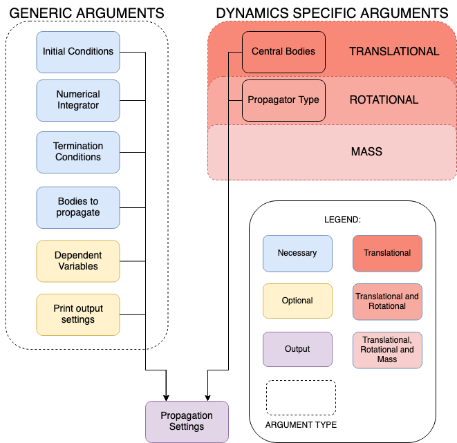
To perform any numerical propagation, propagation settings need to be defined first. To define the propagation settings, you must have created your physical environment first. As the figure shows, there are some input arguments common to all types of single-arc dynamics, while some others are specific to the type of dynamics. On the left there are generic arguments, which is a list of both necessary and optional arguments that must (or can) be provided to the Propagation Settings. On the right, there are dynamics specific arguments. Moreover, for mass dynamics, no additional input is required, whereas for rotational dynamics a propagator must be defined, and for translational dynamics – in addition to the propagator – central bodies need to be defined. More in-depth information about inputs are explained in the dynamic-specific pages linked below.
There are various options in the propagator settings that must (or can) be provided by a user to modify the behaviour before, during and after the propagation. The ones that are common to all dynamics types are described in more detail in the following pages:
List of propagated bodies: the names of the bodies for which the dynamics is to be propagated.
Dependent variables: which quantities to save as output, in addition to the states, described here. These settings are optional (none by default).
Numerical integrator: the solver used to create an approximate solution, described here. This setting is mandatory
Termination conditions: when to terminate the propagation, described here. This setting is mandatory
Processing/output settings: what to print to the terminal before, during and after propagation, and what to do with the numerical results after propagation, both described here. This setting is optional (no terminal output or resetting of environment by default)
The propagation of a given type of dynamics is defined by calling the associated factory function. For the different types of
single-arc dynamics, these factory functions return an object (derived from the
SingleArcPropagatorSettings
class) defining the settings of the propagation. The specifics of how to change the settings for the
different types of dynamics, some of which are specific to the dynamics type (e.g. accelerations for
translational dynamics), and some of which are common to all, are discussed on the specific
pages linked to in the next section
Dynamics types
As previously mentioned, there are a few different types of dynamics that Tudat can numerically propagate:
Translational Dynamics: the translational state of a body is propagated;
Rotational Dynamics: the rotational state of a body is propagated;
Mass Dynamics: the mass of a body is propagated.
Custom Dynamics: an arbitrary user-defined state derivative model, see
custom_state()(typically in the context of a multi-type propagation).
Furthermore, any combination of any number of types of dynamics for any number of bodies can be defined. Therefore, in Tudat we also have:
Multi-type dynamics: more than one dynamical quantity is propagated for a single body;
Multi-body dynamics: only one dynamical quantity is propagated for multiple bodies;
A combination of the two: more than one dynamical quantity is propagated for multiple bodies.
The above list defines different types of dynamics that are propagated over a single continuous arc. Propagation using a multi-arc setup is also supported in Tudat.
Note
For a given type of dynamics, the propagated state can be formulated through a number of different state representations. For the case of translational dynamics, for instance, there are various options besides a simple Cartesian state representation. However, even when using a non-Cartesian state vector, the Cartesian representation still plays a role in calculating, e.g., acceleration models, as well as in defining the initial state. For more information on the role of different state representations, please visit the page Processed vs. Propagated State Elements.