State Estimation
In this section, we discuss the functionality that is required for state estimation in Tudat. Before starting this section, make sure to go through our page on Propagation Setup, since the state estimation function requires the full functionality from state propagation. At the moment, the estimation functionality of Tudat is limited to the use of batch least-squares. A broad range of parameters (initial translational and rotational state; single-, multi- and hybrid-arc states; numerous physical properties of the environment) from a diverse set of available observations is supported. Estimation in Tudat is organized as shown in the figure below.
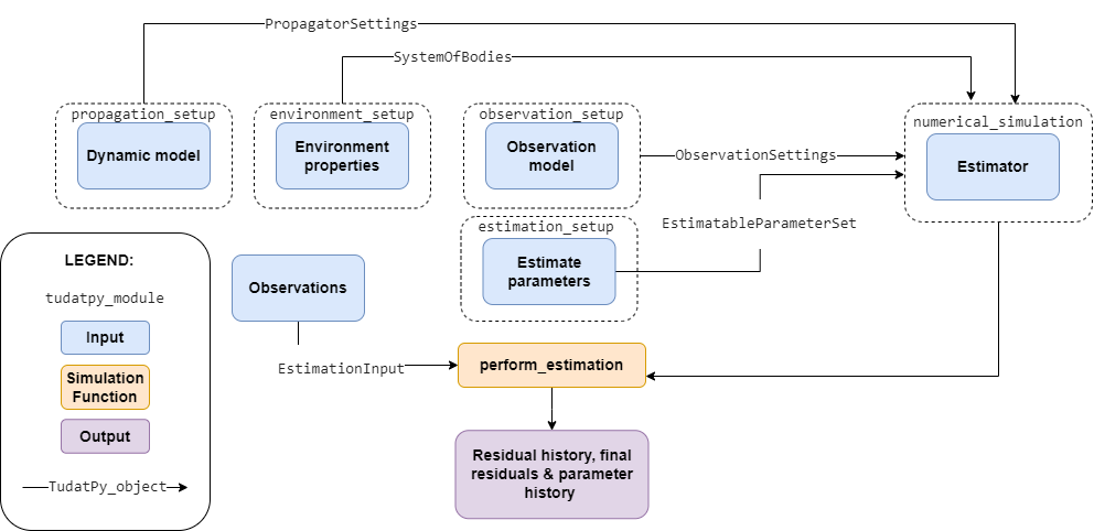
Estimation Inputs
In addition to the inputs required for state propagation, the following needs to be set up to perform an estimation.
Parameter setup: definition of the parameters that are to be estimated, as discussed here in the context of variational equation propagation
Link Ends Setup: define the stations/spacecraft involved in an observation, and define their role for a particular observable (receiver, transmitter, etc.)
Observation Model Setup: define the type and properties of a given observation model, such as range, Doppler, including biases, light time corrections etc.
Providing the observations, including the values of the observables, associated observation times and additional relevant data such as integration time (depending on the observable). This can be done in one of two ways:
Observation Creation For a simulation study, the observations themselves may be simulated inside Tudat
Loading observations: When analyzing real data, you must load these data from the relevant files/database, and convert them to Tudat-compatible data formats.
Estimation Settings: define the a priori knowledge, convergence criteria, etc.. Tudat provides settings and options for either a full estimation, or a covariance analysis only.
Simulation/Analysis & Output
Once all the settings are in place, the solution can be generated: the (simulated) observations can be fit to the dynamical model that has been defined to perform the fitting. Alternatively, the same functionality can be used for a covariance analysis only, in which case no fit is attempted. Details are provided on this page